Mobility Calculation
载流子迁移率通常指半导体内部电子和空穴整体的运动快慢情况,是衡量半导体器件性能的重要物理量。2004年,石墨烯的成功剥离引起了研究人员对于二维材料性质探索的浓厚兴趣。石墨烯、黑磷等二维材料展现出的高载流子迁移率是其中的一个重要研究课题,科研人员在理论计算方面已经做了大量的工作。由于电子在运动过程中不仅受到外电场力的作用,还会不断的与晶格、杂质、缺陷等发生无规则的碰撞,大大增加了理论计算的难度。
目前计算载流子迁移率比较常用的理论是形变势理论和玻尔兹曼输运理论,前者没有考虑电子和声子(晶格振动)以及电子与电子之间的相互作用等因素,计算结果存在一定的误差,但笔者的计算结果与实验值在数量级上是吻合的;玻尔兹曼输运理论的一种计算考虑了电子-声子的相互作用,基于第一性原理计算和最大局域化wannier函数插值方法,借助于 Quantum-ESPRESSO 和 EPW 软件可以完成载流子迁移率计算。缺点是计算量太大,一般的课题组很难承受起高昂的计算费用,另外EPW软件对于二维材料的计算存在部分问题,在其官方论坛也有讨论,计算过程在后续文章中会提到。
本文以形变势理论方法为基础,详细介绍了二维InSe的电子和空穴的有效质量与载流子迁移率的计算方法。
理论基础
基于 Bardeen and Shockley 提出的形变势理论,二维材料载流子迁移率可以根据下式计算:
其中, \(m^{\ast}\) 是传输方向上的有效质量, \(T\) 是温度, \(k_B\) 是玻尔兹曼常数 \(E_1\) 表示沿着传输方向上位于价带顶(VBM)的空穴或聚于导带底(CBM)的电子的形变势常数,由公式 \(E_1 = {\Delta}E/({\Delta}l/l_o)\) 确定, \({\Delta}E\) 为在压缩或拉伸应变下CBM或VBM 的能量变化, \(l_0\) 是传输方向上的晶格常数, \({\Delta}l\) 是 \(l_0\) 的变形量。 \(m_d\) 是载流子的平均有效质量,由公式 \(m_d = \sqrt{m_x^{\ast}m_y^{\ast}}\) 定义。 \(C_{2D}\) 是均匀变形晶体的弹性模量,对于2D材料,弹性模量可以通过公式 \(C_{2D}=2[{\partial}^2E/{\partial}({\Delta}l/l_0)^2]/S_0\) 来计算,其中 \(E\) 是总能量, \(S_0\) 是优化后的面积。
下面对公式中的单位(量纲)做一个简单换算,具体如下:
换算过程:
其中: \(1 V = 1 J/C\) , \(1 J = 1Kg \cdot m^2 / s^2\)
计算与数据处理工具
#! /usr/bin/python
# This program reads in base vectors from a given file, calculates reciprocal vectors
# then writes to outfile in different units
# LinuxUsage: crecip.py infile outfile
# Note:  the infile must be in the form below:
#   inunit  ang/bohr
#   _begin_vectors
#     46.300000000   0.000000000   0.000000000
#      0.000000000  40.500000000   0.000000000
#      0.000000000   0.000000000  10.000000000
#   _end_vectors
#
# Note: LATTICE VECTORS ARE SPECIFIED IN ROWS !
def GetInUnit( incontent ):
    inunit = ""
    for line in incontent:
        if line.find("inunit") == 0:
            inunit = line.split()[1]
            break
    return inunit
def GetVectors( incontent ):
    indstart = 0
    indend = 0
    for s in incontent:
        if s.find("_begin_vectors") != -1:
            indstart = incontent.index(s)
        else:
            if s.find("_end_vectors") != -1:
                indend = incontent.index(s)
    result = []
    for i in range( indstart + 1, indend ):
        line = incontent[i].split()
        result.append( [ float(line[0]), float(line[1]), float(line[2]) ] )
    return result
def Ang2Bohr( LattVecAng ):
    LattVecBohr = LattVecAng
    for i in range(0,3):
        for j in range(0,3):
            LattVecBohr[i][j] = LattVecAng[i][j] *  1.8897261246
    return LattVecBohr
def DotProduct( v1, v2 ):
    dotproduct = 0.0
    for i in range(0,3):
        dotproduct = dotproduct + v1[i] * v2[i]
    return dotproduct
def CrossProduct( v1, v2 ):
    # v3 = v1 WILL LEAD TO WRONG RESULT
    v3 = []
    v3.append( v1[1] * v2[2] - v1[2] * v2[1] )
    v3.append( v1[2] * v2[0] - v1[0] * v2[2] )
    v3.append( v1[0] * v2[1] - v1[1] * v2[0] )
    return v3
def CalcRecVectors( lattvec ):
    pi = 3.141592653589793
    a1 = lattvec[0]
    a2 = lattvec[1]
    a3 = lattvec[2]
    b1 = CrossProduct( a2, a3 )
    b2 = CrossProduct( a3, a1 )
    b3 = CrossProduct( a1, a2 )
    volume = DotProduct( a1, CrossProduct( a2, a3 ) )
    RecVec = [ b1, b2, b3 ]
    # it follows the definition for b_j: a_i * b_j = 2pi * delta(i,j)
    for i in range(0,3):
        for j in range(0,3):
            RecVec[i][j] = RecVec[i][j] * 2 * pi / volume
    return RecVec
def main(argv = None):
    argv = sys.argv
    infilename  = argv[1]
    outfilename = argv[2]
    pi = 3.141592653589793
    bohr2ang = 0.5291772109253
    ang2bohr = 1.889726124546
    infile  = open(infilename,"r")
    incontent = infile.readlines()
    infile.close()
    inunit = GetInUnit( incontent )
    LattVectors = GetVectors( incontent )
    # convert units from ang to bohr
    if inunit == "ang":
        LattVectors = Ang2Bohr( LattVectors )
    # calculate reciprocal vectors in 1/bohr
    RecVectors = CalcRecVectors( LattVectors )
    # open outfile for output
    ofile = open(outfilename,"w")
    # output lattice vectors in bohr
    ofile.write("lattice vectors in bohr:\n")
    for vi in LattVectors:
        ofile.write("%14.9f%14.9f%14.9f\n" % (vi[0], vi[1], vi[2]))
    ofile.write("\n")
    # output lattice vectors in ang
    convfac = bohr2ang
    ofile.write("lattice vectors in ang:\n")
    for vi in LattVectors:
        ofile.write("%14.9f%14.9f%14.9f\n" % (vi[0]*convfac, vi[1]*convfac, vi[2]*convfac))
    ofile.write("\n")
    # output reciprocal vectors in 1/bohr
    ofile.write("reciprocal vectors in 1/bohr:\n")
    for vi in RecVectors:
        ofile.write("%14.9f%14.9f%14.9f\n" % (vi[0], vi[1], vi[2]))
    ofile.write("\n")
    # output reciprocal vectors in 1/ang
    convfac = ang2bohr
    ofile.write("reciprocal vectors in 1/ang:\n")
    for vi in RecVectors:
        ofile.write("%14.9f%14.9f%14.9f\n" % (vi[0]*convfac, vi[1]*convfac, vi[2]*convfac))
    ofile.write("\n")
    # output reciprocal vectors in 2pi/bohr
    convfac = 1.0/(2.0*pi)
    ofile.write("reciprocal vectors in 2pi/bohr:\n")
    for vi in RecVectors:
        ofile.write("%14.9f%14.9f%14.9f\n" % (vi[0]*convfac, vi[1]*convfac, vi[2]*convfac))
    ofile.write("\n")
    # output reciprocal vectors in 2pi/ang
    convfac = ang2bohr/(2.0*pi)
    ofile.write("reciprocal vectors in 2pi/ang:\n")
    for vi in RecVectors:
        ofile.write("%14.9f%14.9f%14.9f\n" % (vi[0]*convfac, vi[1]*convfac, vi[2]*convfac))
    # close
    ofile.close()
    return 0
if __name__ == "__main__":
   import sys
   sys.exit(main())
二维InSe有效质量计算过程
建模
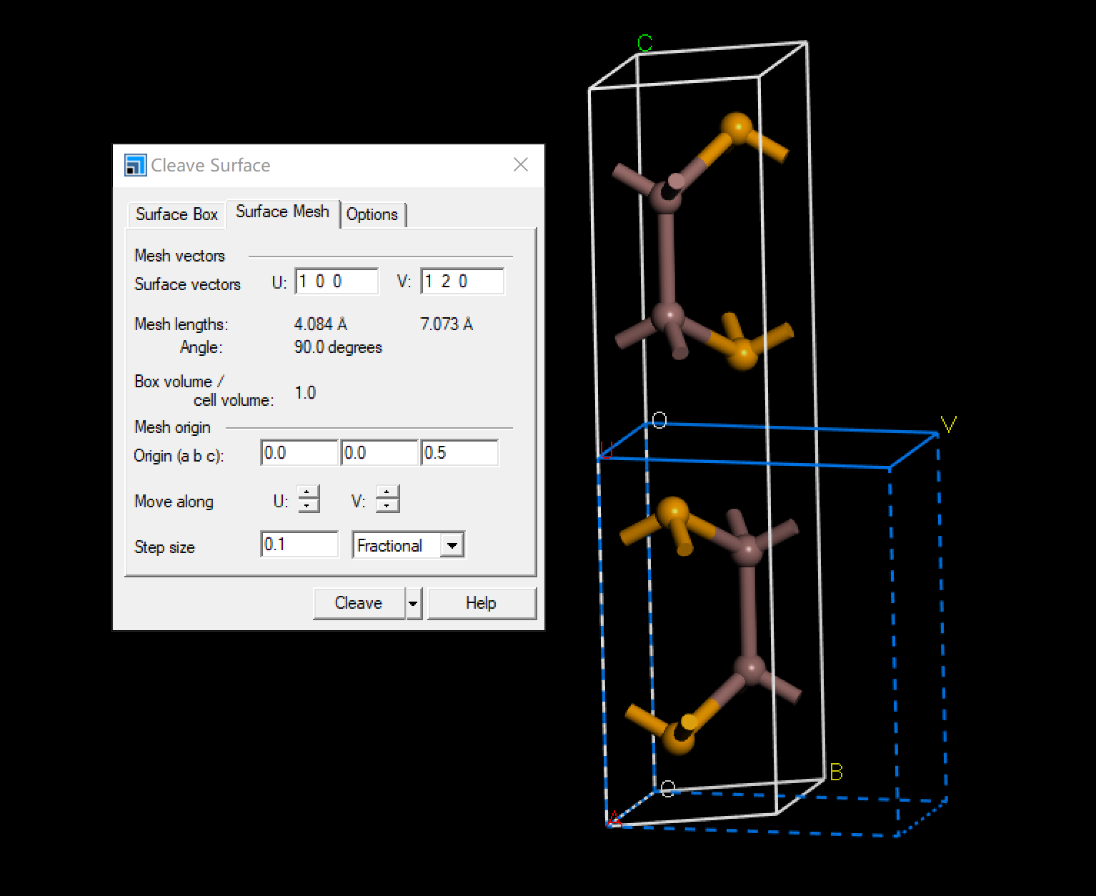
由于计算过程中需要对二维InSe施加应变,但二维InSe原胞是六角结构,不容易施加应变。但是侯柱峰老师讲了对石墨烯原胞施加应变的方法,笔者认为虽然可行,但过于繁琐,故不采用此法。我们可以利用根号建模的方法讲六角结构InSe原胞变为方形结构的InSe超胞,然后施加应变可大大提高操作效率,但计算量的增加在可接受范围之内。下面给出关键的建模步骤,更多的根号建模部分可参考我的往期博客文章。
能带计算
结构优化
SYSTEM = InSe
ISTART = 0
NWRITE = 2
PREC   = Accurate
ENCUT  = 500
GGA    = PE
NSW    = 200
ISIF   = 3
ISYM   = 2
IBRION = 2
NELM   = 80
EDIFF  = 1E-05
EDIFFG = -0.01
ALGO   = Normal
LDIAG  = .TRUE.
LREAL  = .FALSE.
ISMEAR = 0
SIGMA  = 0.05
ICHARG = 2
LWAVE  =  .FALSE.
LCHARG = .FALSE.
NPAR   = 4
Monkhorst Pack
0
Gamma
 11   7   1
.0   .0   .0
  Se   In
  1.000
       4.083622259999999      -0.000000000000001       0.000000000000000
       0.000000000000000       7.073041233239241       0.000000000000000
       0.000000000000000       0.000000000000000      25.377516849029359
  Se   In
  4   4
Direct
  0.5000005000000000   0.1666665000000000   0.5271404971815050   !Se
  0.0000004999999997   0.6666665000000004   0.5271404971815050   !Se
  0.5000005000000000   0.1666665000000000   0.3152396685456632   !Se
  0.0000004999999997   0.6666665000000004   0.3152396685456632   !Se
  0.4999995000000003   0.8333335000000002   0.4767849697227853   !In
 -0.0000005000000000   0.3333335000000000   0.4767849697227853   !In
  0.4999995000000003   0.8333335000000002   0.3655951960043828   !In
 -0.0000005000000000   0.3333335000000000   0.3655951960043828   !In
cat Se/POTCAR In_d/POTCAR > POTCAR
100
010
000
静态自洽
SYSTEM = InSe
ISTART = 0
NWRITE = 2
PREC   = Accurate
ENCUT  = 500
GGA    = PE
NSW    = 0
ISIF   = 2
ISYM   = 2
IBRION = -1
NELM   = 80
EDIFF  = 1E-05
EDIFFG = -0.01
ALGO   = Normal
LDIAG  = .TRUE.
LREAL  = .FALSE.
ISMEAR = 0
SIGMA  = 0.05
ICHARG = 2
NPAR   = 4
Monkhorst Pack
0
Gamma
 21   13   1
.0   .0   .0
cp CONTCAR scf/POSCAR